Historical Presidential Tweets

1. Background
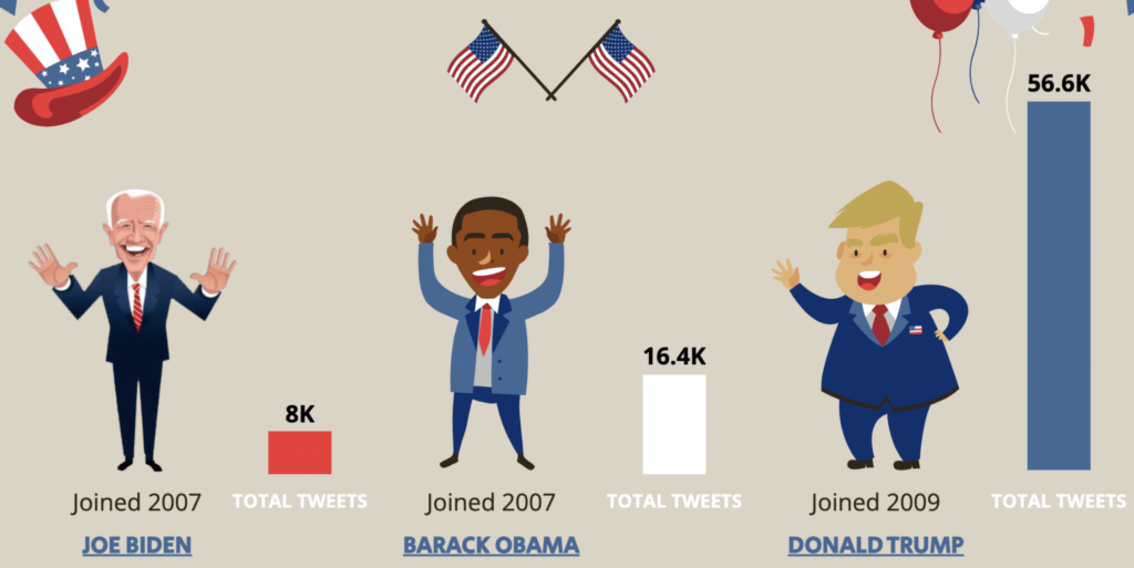
Donald Trump is the most prolific president when it comes to tweeting. He left behind a treasure trove of data, so I wanted to take a historical look at how he used Twitter and what was said.
The goal of this project is to build a model using topic modeling, sentiment analysis, and time series to gain insight into Donald Trump’s Twitter history.
Notes:
- This project is not intended to represent any individual’s personal political beliefs.
- This project was completed before company formerly known as ‘Twitter’ was renamed ‘X’. To pay homage to the bird I will be using the original ‘Twitter’ name.
2. The Data
I download a .csv file of Donald Trump’s entire Twitter history (2009-2021) from thetrumparchive.com. The data was originally scraped using ‘Tweet Scraper’ by the sites creator. The dataset has 56,571 rows and 9 columns.
Features:
- tweet text
- isRetweet
- date/time
- likes
- isDeleted
- isFlagged
- id
- retweets
- device
3. Methodology
I used natural language processing techniques to categorize topics for tweets, looked at topics over time, generated sentiment scores for each tweet, and looked at sentiment over time.
Tools Used:
- EDA: Excel
- Regular Expression
- datetime
- Data Manipulation: Numpy, Pandas
- Plotting/ Visualizing: matplotlib, seaborn, Tableau
- Modeling: sklearn, CountVectorizer
- NLP: NLTK, CorEx
- Sentiment Analysis: vaderSentiment
					%reset -fs

import pandas as pd
import numpy as np
from sklearn import metrics
import matplotlib.pyplot as plt
import matplotlib
import seaborn as sns
import re
import string
from datetime import datetime as dt
from sklearn.feature_extraction.text import CountVectorizer
from sklearn import datasets
from corextopic import corextopic as ct
from vaderSentiment.vaderSentiment import SentimentIntensityAnalyzer

matplotlib.use('TkAgg')
%matplotlib inline
pd.set_option("display.max_colwidth", 1)
4. Workflow
4.1. Text Processing
After initial EDA in Excel there was more to do within Python. Because the data is scraped tweets there are some random characters that appear in the data and other weird things to work through.
To begin with it wasn’t apparent at first but the encoding for the .cvs file had to be set to ‘utf-8’ to get the dataset to show correctly.
df = pd.read_csv('tweets_01-08-2021.csv', encoding='utf-8')
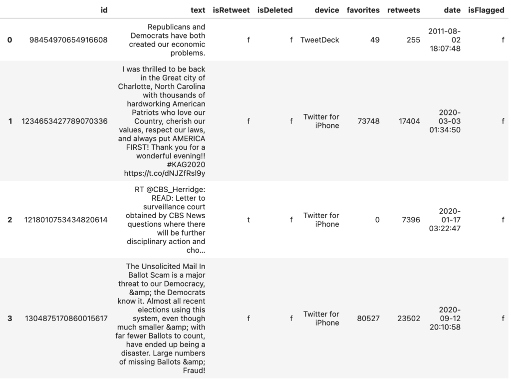
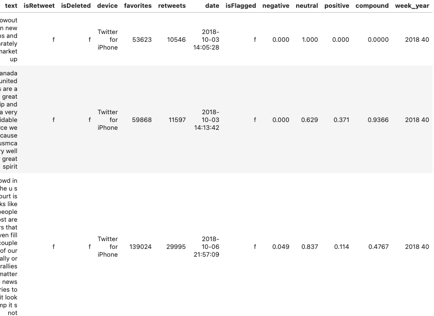
Here is an example of what the imported data looks like.
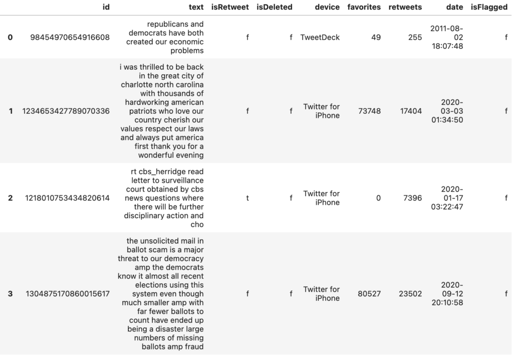
It was necessary to remove numbers, URL’s, capital letters, and punctuations from all tweets. This was done using Regular Expression.
					# Text preprocessing steps - remove numbers, URL, captial letters and punctuation
alphanumeric = lambda x: re.sub('\w*\d\w*', ' ', x)
punc_lower = lambda x: re.sub(r'[^\w\s]', ' ',str(x).lower())
no_url = lambda x: re.sub(r'http\S+', '', x)
clean = lambda x: x.replace('\n', '')
english_only = lambda string: re.sub(r'[^\x00-\x7f]', "", string)

df['text'] = df.text.map(alphanumeric).map(no_url).map(punc_lower).map(clean).map(english_only)
Since certain tweets were only URL’s, and those were removed, I was left with empty cells. So the next step was to fill the empty cells with Null values and then drop them since they won’t be needed.
					df['text'] = df['text'].apply(lambda x: x.strip()).replace('', np.nan) # fill empty cells w/ Null values
df = df.dropna() #drop null rows
Formatting of the ‘date’ using datetime.
df["date"] = pd.to_datetime(df.date , format="%Y/%m/%d %H:%M:%S") #create date_time column
4.2. Topic Modeling
For topic modeling, text preprocessing and feature extraction is set up on ‘text’.
I tried several types of modeling:
- LSA
- NMF w/ TF-IDF
- CorEx w/ TF-IDF
- CorEx w/ CountVectorizer
I got the best results using CorEx w/ CountVectorizer for clear topic categories. ‘CountVectorizer’ converts the text data into a numerical format suitable for machine learning models and I will have a binary document-term matrix (doc_word) and a list of feature names (words) that can be used as inputs.
					vectorizer = CountVectorizer(max_features=20000,
                             stop_words='english',
                             token_pattern="\\b[a-z][a-z]+\\b",
                             binary=True, max_df=0.8,ngram_range=(1, 4))

doc_word = vectorizer.fit_transform(df.text)
words = list(np.asarray(vectorizer.get_feature_names()))
For the topic modeling ‘Corex’ was used to train the model and extract latent topics. The topics represent groups of words that tend to co-occur in the documents and can provide insights into the main themes or subjects present in the text corpus. It was necessary to iterate on generating the topics to see what words to use as (anchors) and the create topics that are easy to identify.
					topic_model = ct.Corex(n_hidden=7, words=words, seed=1)
topic_model.fit(doc_word, words=words, docs=df.text,
               anchors= [['news'],['military'],['democrats'],['hillary', 'obama','barackobama'],
                         ['rally']], anchor_strength=3)
					# Print all topics from the CorEx topic model
topics = topic_model.get_topics()
for n,topic in enumerate(topics):
    topic_words,_,_ = zip(*topic)
    print('{}: '.format(n) + ','.join(topic_words))
I used the next line of code to look at the top tweets of each topic. Here is an example of the top 2 tweets in topic #3.
topic_model.get_top_docs(topic=3, n_docs=2)
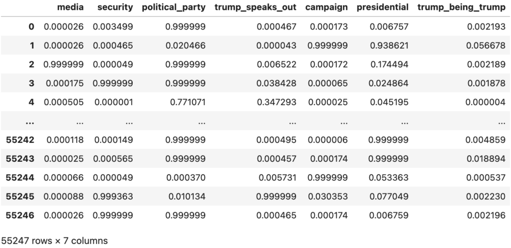
A topic prediction matrix was generated using the previously trained ‘Corex’ topic model and organized the results into a dataframe. Each row represents a tweet, and each column represents a topic. This allows for an individual tweet to be checked to verify that it belongs in a given topic. The topics were also give names:
- Media
- Security
- Political Party
- Trump Speaks Out
- Campaign
- Presidential
- Trump Being Trump
					df_probability = pd.DataFrame(topic_model.p_y_given_x)

#rename topics
df_probability = df_probability.set_axis(['media', 'security', 'political_party', 'trump_speaks_out', 'campaign',
                                           'presidential','trump_being_trump'], axis=1, inplace=False)
4.3. Sentiment Analysis
Sentiment Analysis was run using ‘vaderSentiment’ and the scores were added to the dataframe for each tweet. The dataframe was then split by week and the compound Sentiment score (used as an overall indicator) was averaged for each week. I will go through each of these steps.
Initializing an instance of the ‘SentimentIntensityAnalyzer’ class.
analyzer = SentimentIntensityAnalyzer()
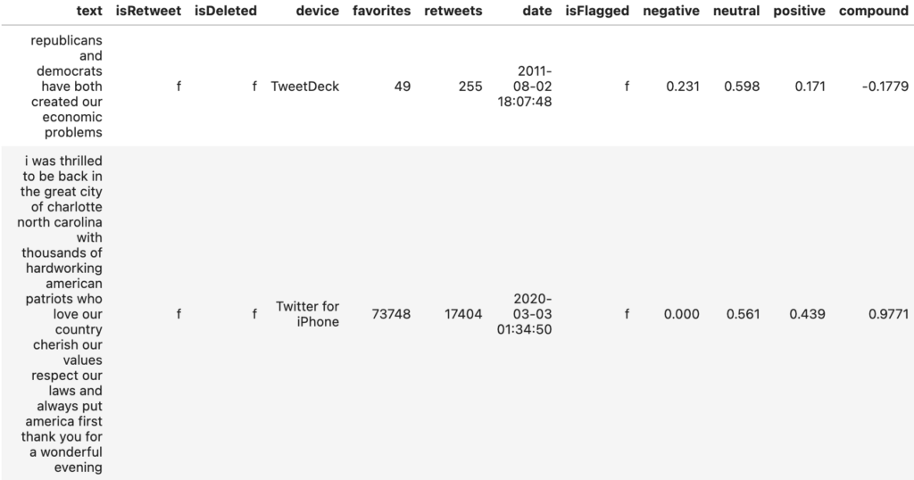
Next a function was created to get the sentiment scores and add them to the dataframe for each corresponding tweet.
The compound sentiment score combines the ‘positive’, ‘negative’, and ‘neutral’ sentiments into a single value. You can use these scores to determine the overall sentiment of a piece of text, with the ‘compound’ score being a commonly used metric for this purpose.
					def get_polar_score(x):
        """
        create sentiment score & break by index
        """
        polar_dict = analyzer.polarity_scores(x)
        negative = polar_dict['neg']
        positive = polar_dict['pos']
        neutral = polar_dict['neu']
        compound = polar_dict['compound']
        return negative, neutral, positive, compound
					# add sentiment score columns to df
df['negative'] = df.text.apply(lambda z: get_polar_score(z)[0])
df['neutral'] = df.text.apply(lambda z: get_polar_score(z)[1])
df['positive'] = df.text.apply(lambda z: get_polar_score(z)[2])
df['compound'] = df.text.apply(lambda z: get_polar_score(z)[3])
To view tweets by week a week of the year variable was created called ‘week_year’.
					# create week_year column
df['week_year']= df.date.dt.strftime('%G %V')
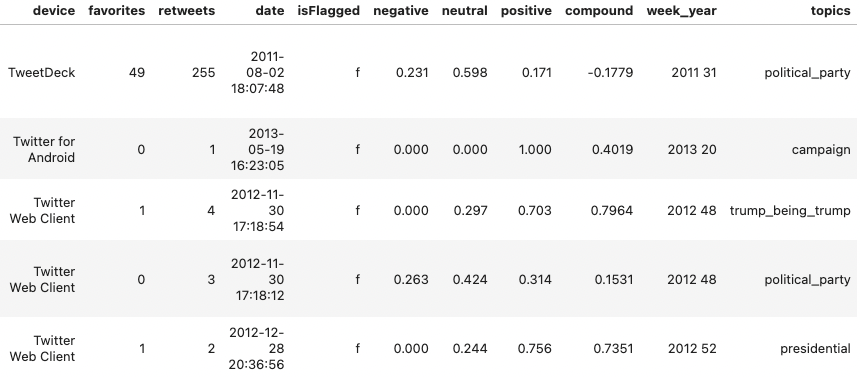
A ‘topics’ variable was created and added to the dataframe for the final bit of feature engineering.
					# create topic column, with max probability topic
df['topics'] = df_probability.iloc[:,-7:].idxmax(axis=1)

# convert Nan values to 'other'
df['topics'] = df['topics'].fillna('other')
5. Evaluate & Interpret
In this section I took a look into Donald Trump’s tweets over time using the compound sentiment score, individual tweets, and research into what was happening politically around points of interest. The charts for this section were created in Tableau.
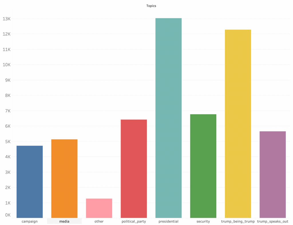
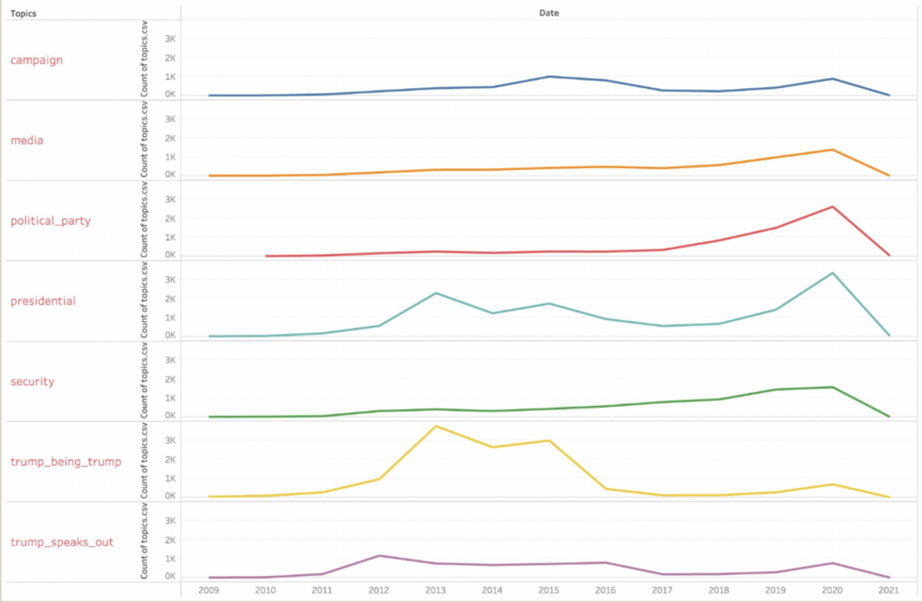
In this first chart we see that the topics ‘Trump Speaks Out’ and ‘Trump Being Trump’ contained similar tweets, but interestingly even though ‘Trump Being Trump’ was the last topic generated it had the second most tweets of any topic.
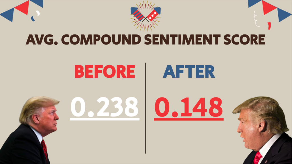
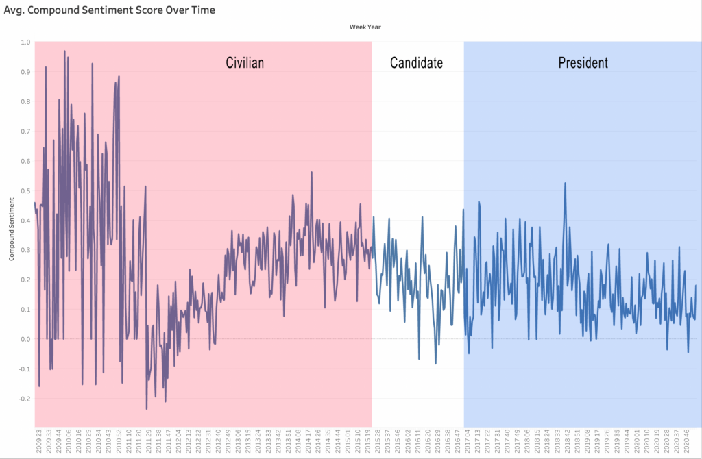
This is the average Compound Sentiment score for before and after Donald Trump became president. Overall Trump’s tweets were positive, but somewhat less after he became president.
For topics over time we see spikes with a similar slope in tweets for the topics ‘Presidential’, ‘Trump Speaks Out’, and ‘Trump Being Trump’. This timeline (2011-2017) coincides with when Donald Trump started to speak out on Twitter and through his candidacy for president. In the second half of his presidency (2019-2021) we see a spike in the amount of tweets for all topics.
In the average compound sentiment over time we see Trump’s tweets displayed overtime, grouped together by week, and shows when he was a civilian, candidate, and president.
Notable point in the charts timeline:
Civilian
- In the beginning of his tweet history we see big jumps in +/- for the tweets. This is because Donald Trump is tweeting less but when he does the tweets tend to be very positive or negative.
- The highest positive point (0.971) of Trumps Twitter history happens in this time, and it’s a tweet wishing everyone a merry Christmas.
- Trumps most negative point (-0.236) happens while he is still a civilian. Several things coincide with this timeframe (year 2011, week 27).
- July 4- 2011 Fox News gets Hacked.
- July 6- First “Twitter Presidential Town Hall” hosted by Jack Dorsey (co-founder and former CEO of Twitter) with President Obama. This is the first time we see Trump’s raw and unfiltered political critique of Obama.
- Over the following few months Trump overtly criticizes Obama and Republicans. This is when we see his Twitter following start to swell.
- It could be said that this time period is when Trump finds his Twitter voice.
Candidate
- For this period the trend slopes negative. Trump is running attack ads on opponents is getting kind of nasty.
President
- The lowest negative point (-0.049) for a tweet, during this period, happens at the beginning of his presidency. Things of note happening around this timeframe (week 5, year 2017):
- Trump goes on an executive order signing spree.
- Feb. 3, 2017- District Court temporarily blocks order to temporarily block immigration from seven Middle Eastern nations.
- Feb. 5- 9th Circuit court denies request from Trump administration to immediately reinstate a travel ban.
- Trump refers to Elizabeth Warren as Pocahontas. (Trump is lashing out everywhere cause he is not getting his way on everything.)
- The highest positive point (0.526) for tweets during his presidency happens in the middle of this period. Of note around this timeframe:
- Oct. 5, 2018- The Senate confirms Brett Kavanaugh to the Supreme Court.
6. Key Takeaways & Further Steps
- Overall Donald Trump’s tweets are not super negative.
- He praises quite a bit.
- The number of topics he tweets about grow in the second half of his presidency.
- Earlier tweets vary greatly between positive and negative.
- Unfiltered Trump shows up around July 6, 2011.
- He is slightly more positive before his presidency.

